Percentiles in Webi

Can this be possible in Webi using same logic as in this blog here?I can’t understand the part where 5, 25 and so forth percentiles values are shown (the last block). Can anyone guide me with this? http://blogs.adatis.co.uk/blogs/david/archive/2011/06/24/calculating-percentile-brackets-using-sql-server-2008.aspx


excel-c-us (BOB member since 2011-09-20)

Hi

There is a percentile function in Webi where if you have a measure say [revenue] and you want to know the value of the 25% percentile you use,

percentile([revenue],0.25)

and similarly for other values

regards

AL


agulland :uk: (BOB member since 2004-03-17)

I agree there is this function. But it doesn’t give me same values as I have to bring on my reports. Secondly in the last block he has brought together all the values closest to percentiles. So basically I don’t need to show exactly 10 or 20 percentile, it is maximum value in close to or equal to 10, 20 and 50 percentile.


excel-c-us (BOB member since 2011-09-20)

Create the logic in the database or via a derived table in the universe, then report of that. Webi itself does not support any Looping such as WHILE Condition = TRUE DO… END.
Crystal Reports does.


Andreas :de: (BOB member since 2002-06-20)

To calculate percentiles you need to work with dimension objects
ie retrieve Revenue as a dimension

Mick


mikca :australia: (BOB member since 2005-12-16)

Thanks guys. I know its tricky. I have emulated half way its done in excel in my environment. I’ll share it here for you guys to see if there is anything that can be done beyond this point.

Column with decimal values has simple formula Revenue/Sum(Revenue) in ([Year]) which gives me sum of 1 for each column in crosstab in second image.

Column with percentages is where I used Runningsum([Var]). What I need from here is simply “Quarter” and “decimal value” that corresponds to percentage. So lets say 2004/Q3 has value of 0.17 which corresponds to 78%. So if I had a 80 percentile it this would be my value because this is closest value to 80. So I just need to show to Quarters and Decimal values for 10, 25, 40, 75, 90 percentile which would be max for each quarter in a year and I dont want all the other values such 33% and 61%.
Eventual Result should be the way it is third block
Thought if I could solve it this way, would save me time to create a query in universe.
Running Sum.JPG
Capture3.JPG
max.JPG


excel-c-us (BOB member since 2011-09-20)

Hi

I don’t know the business context of what you want to use these Percentiles for but I would caution against using a number that is closest to the true percentile value and stating that as the percentile rather than the percentile itself.

The author of that blog you reference says it is better to determine nearest value rather than actual but I would disagree on this point. Let me explain by example.

Consider a set of exam results where the marks are out of 20. If there are many results and they are evenly spread from 0 to 20 then we expect the score for the 50% percentile to be about 10 (half of 20).

However if for some weird reason there isn’t an even spread of scores but instead a lot of very high scores (all 17 or above say) and then also a lot of very low scores (all 2 or below say) then this will also give the 50% percentile as about 10 however the nearest value to 10 will be 17. So you can then say “I’m a very good teacher as half my class score 17 or over” which is technically true but this hides the fact that the other have got really bad scores!

Statistical measures such as Percentile, and mean, median, mode, standard deviation etc, are used to describe a set of data and you should be careful that they don’t hide or obscure unusual features such as the example above.

Like I said, I don’t know what you are wanting to use these percentiles for in a business scenario but I think using the Percentile function may in fact be what you want rather than determining the number nearest the percentile value - and of course much easier to calculate!

something to think about, regards

AL


agulland :uk: (BOB member since 2004-03-17)

agulland. Thanks for your response. I myself am perplexed as to why they want to calculate this as a nearest or equal value to percentile. But this is what is required by business at this point. If I calculate percentiles even though they are true values of percentiles, they won’t show values that are required in report. So my only hope is to somehow display the values as I showed in my example above. Is there a way to show nearest value of each percentile for each of the percentiles in the crosstab format as I showed in last block of examples above?


excel-c-us (BOB member since 2011-09-20)

Gah, if it wasn’t for those pesky business users our lives would be so much easier!

OK so if they aren’t willing to change their mind then I think we may be able to get closest value. Below is off the top of my head and I haven’t tried it but I think it’ll work.

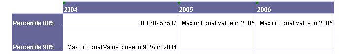
The idea is to create a new dimension that groups the values into the percentiles, e.g. all values less then the 10% percentile are assigned value “10%”, values between the 10% and 20% percentile are assigned “20%”. Then we can use max and min functions (or maybe First and Last) to get the two values closest to the actual percentile value - max of one range and min of the next. Then determine which is closer and use that.

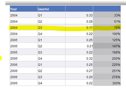
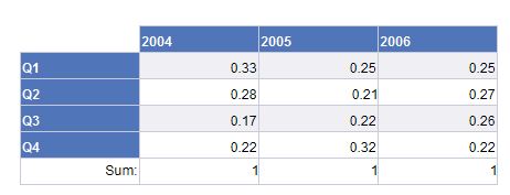
Start with a table of all data and initially just use one percentile - 50% say - once we get this working we can extend for all percentiles.

Add a new column and add Percentiles formula to this column and use calculation contexts so tha the percentile is calculated for the whole table and not just the row, something like:

=Percentiles([measure];0.5) In Block

Add another column and using an If formula label the rows as “0%” or “50%” if the measure value is less that the 50% percentile or not. Convert this formula to a dimension “Percentile Range”.

Add two more columns and in these use the Max function to get the max value below the 50% percentile and similarly use the Min function to get the first value above 50% percentile using the dimension we just created.

=Max([measure]) where ([Percentile Range]="0%")
=Min([measure]) where ([Percentile Range]="50%")

Now you can compare these values to the actual percentile to determine the value closest. Something like:

=if Max([measure]) where ([Percentile Range]="0%") - Percentile[measure;0.5) < Min([measure]) where ([Percentile Range]="50%") then Max([measure]) where ([Percentile Range]="0%") else Min([measure]) where ([Percentile Range]="50%") 

For more than one percentiles you’ll need to use a lot of nested if statements but I think it’ll work. Once you get this working you can then remove the additional ‘working’ columns. You can probably remove the measure column and the data will aggregate up but you’ll need to keep the new [Percentile Range] dimension.

AL


agulland :uk: (BOB member since 2004-03-17)

Thanks agulland. Appreciate your effort. Let me understand it and implement it and I’ll reply here regarding the outcome. Thanks again.


excel-c-us (BOB member since 2011-09-20)